How a robot finds its location based on what it ‘sees’
So how can a robot ‘see’?

Fundamental techniques for navigation
If you were sending a robot to explore Mars, what technology would you use to help that robot navigate independently?
In order for that robot to navigate independently, it needs to do a few things — first, it needs to gather information, and secondly, it needs to know how to ask itself questions. Lastly, it needs a way to come up with a solution.
The robot needs to be able to ask itself:
“Where am I? Where am I going and how do I get there?”
This is the key question that NASA’s rover, Curiosity, asked itself on Mars. For humans, we have eyes and a brain to process sensory information, so usually we jump to finding a solution. But for a robot, we have to build from scratch. What technologies are available for it to understand its surroundings? Before it even moves around, how can a robot see?
What kind of robot do we need?
In robotics, the NASA’s Curiosity Rover classifies as a mobile (not-fixed to one location) and autonomous (can move without human control) robot. Drones with autopilot and self-driving cars also belong to this family.
In this article, I will only look into the visual approach for robots to gather sensory data on its environment. This means our robot has a camera installed that serves as its eyes. We will see how this camera-equipped robot can get clues of where it is, and even build a map solely based on what it sees.
What does “a robot know where it is” mean?
The short answer is:
- A robot can pinpoint its location on a given map;
- and know which direction it is facing
Let’s start with how we as humans locate ourselves. We would first look around and search for landmarks that we can find on a map we’re holding. In the city, we’d probably look for famous buildings, shops or crossroads around us and we look for the corresponding symbols that them on the map (bank, toilet, etc.). Based on these symbols being in a matching position to what we see, we can roughly locate ourselves on the map. If we wanted to be precise, we could pull out laser pointers, a compass, and use some trigonometry.

How a robot finds itself on the map
A robot can find itself the same way humans do:
- Look for nearby landmarks;
- Identify landmarks on the map;
- Use the known position of landmarks to deduce its position and orientation
The difference is that a camera-equipped robot needs to be told how to recognize the things on the map it has. So how does a robot understand what it’s seeing?
We humans see an image as a composition of objects that we give meaning.
To a robot, an image as raw data is just a grid of digits.
A robot’s “eyes”, its camera, may take in visual information, but the robot needs to know how to turn those 0’s and 1’s into meaning? It does not know how to identify an apple, a rock or a building.
Let’s put aside the idea of “understanding” the image. Is there a way to “cheat” and have the robot not understand the image while still being able to pick some landmark to search on its own map? The answer is: yes.
Robots using the visual approach can locate themselves without “understanding” the visuals they’re taking in.
If we use the image features as landmarks, and the map consists of a set of image features associated with a robot’s position information, the robot can locate itself. I’ll explain below.
Using image features to identify landmarks
So what is an image feature? Before answering this question, let’s think about what a landmark is.
From Wikipedia,
“A landmark is a recognizable natural or artificial feature used for navigation, a feature that stands out from its near environment and is often visible from long distances.”
In other words, a landmark object looks different from its surroundings — usually due to its distinguishable size or height.
An image feature has the same characteristic as landmark, it is a small region of the image that looks different from its surroundings. It could be the value inside that region that is much larger or smaller than its surroundings. And it is not difficult to realize that image features tend to be found at the dots/corners/vertices of an object, as those areas have sharp change of image value in all directions.

Figure 3a. Eiffel Tower is an example of good landmark as it is unique and able to stand out from the surrounding environment.

Figure 3b. In contrast, houses in the estate are bad landmarks. Given only the facade of a house, we won’t know which house that facade belongs to.
What is considered good features and bad? An example.


Figure 4. The images above are original images, and the images underneath show the parts of the image considered as good identifying features (Red regions imply good features and blue regions imply bad features).
A good image feature that can serve as a landmark would ideally have the same part of an object with the same image feature no matter how that object is being captured by the camera. We would want that detected image feature to remain unchanged even if there is a change in viewing angle and/or change in lighting conditions.
It is very difficult to capture an ideal image feature, however there are ways to practically engineer an image feature that will result in very similar image feature even though there is a change in object size or the image is rotated.
To engineer an image feature, we want to know two things:
- how to find the feature on an image; and
- how to describe it, for example in a matrix

Figure 5. To illustrate what image features and its descriptors look like, we can run a SIFT (Scale-Invariant Feature Transform) [⁴]detector and overlay the detected features with the illustration of descriptors on top of an original image. The yellow circles indicate the location of the features. The green 4x4 grids show the image patch being used to compute the descriptors. The orientation of the grid lets us use the orientation of the feature and the arrows inside a grid showing us the local orientation inside an image patch. Unlike what we are going to discuss in the following passage, instead of describing an image feature solely with pixel values of the image patch, a SIFT descriptor stores the gradient/orientation information of the image feature. This makes a SIFT feature less prone to change in lighting condition.
How to Identify Image features?
One of the ways to search for feature on an image is to look for a sharp change in neighboring pixels for all directions[¹].

Figure 6. Image showing the RGB value of a pixel on an image. When we zoom in an image to a small region, we will see agrid of colored squares.
It would be perfect if we could take the picture of same object from the same distance each time. However if we take a picture with various distances to the object, we will find that we are getting a quite different set of feature for each picture. As we’re varying the distance to object, the size of object being captured is going to change; the closer we take a picture, the bigger the size of the object appears in the image. As we zoom in, some corners will not be considered as corners anymore.
Similarly, if we move away from an object, some part of the object, say a spot, which is too big to consider as corner before will then become a corner. All in all, image feature detection based on local sharp change of pixel is object-size-specific. When we find features in this way, it is better to vary the size of image to make sure we have cover image features which are corresponding to different object size as well. [²]
Describing an image feature
Okay, now we know how to find image features and we can locate them in an image, what’s next? After detecting an image feature, we need to come up with a way to describe it, meaning record how the feature looks. The most straight forward way probably is, draw a 7x7 square centered at the image feature, and use those 49 pixel values inside the square as an descriptor of that feature. If we want the same object but with different color being described by the same (or at least similar) way, instead of storing the 7x7 image patch with all the RGB value, we could use the greyscale value [²].

Figure 7. Illustration shows how to describe an image feature using image patch. Basically we just need to crop a small area of image near the image feature (here is a 15x15 image patch), convert it to grey scale and store the pixel values in a pre-defined order (here is from left to top and from top to bottom.)
Once we have crafted a descriptor for each image feature, we may start to think about how to compare two image features to tell whether they look similar.
We can do this by subtracting one descriptor from the other one (which is calculating 49 subtractions if we are using 7x7 image patch as descriptor), takes the absolute value[³] and then sum up the difference. We have a name for this — SAD (Sum of Absolute Difference).
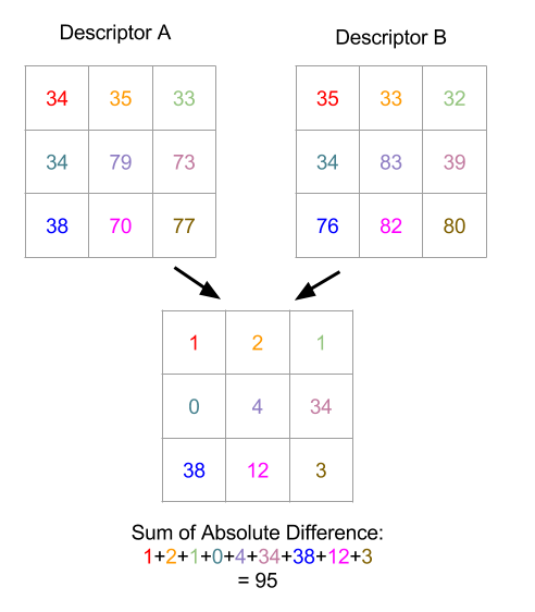
Figure 8. Illustration showing how SAD between 2 3x3 image patches are calculated. First the absolute difference is computed between pixels on the same location (they are having the same color), finally we just need to sum those differences up.
So what does it mean if the SAD value between two descriptors is small? That means two descriptors look similar — the SAD value between two identical descriptors is zero. Hence we could use the SAD value to determine the similarity of image features. And we could pick a threshold value, when the SAD value between two features are lowered than that value (such as 100), we could consider those two features are practically the same.
What if the image is taken in a different angle?
Rotation invariant descriptor
Now, imagine two images. One of them is rotated 30 degrees further from the other one. We could probably find the same set of image features among these two images. However it could result in a very different image descriptors between the feature pair, and this is no good, as that are actually referring to the same part of object. To solve this problem, we should find a way to determine the orientation of an image. And we could do this by computing the gradient images.
∑
Gradient image is describing how an image is changing. It is very easy to compute which is just computing the difference between neighboring pixel’s greyscale value. Each gradient image’s pixel has two components, x and y. The x component is showing how a pixel is changing horizontally, which is the different between the right pixel and the left pixel; the y component is showing how a pixel is changing vertically and it is computed by the difference between the pixel above and the pixel below.
So each pixel of the gradient image is actually telling us how strongly a pixel is changing in both horizontal and vertical directions. By trigonometry, we could compute orientation (the angle, which is arc-tangent of vertical change divided by horizontal change) for each pixel. Similarly, we could sum up all the x-components and y-components of an gradient image respectively and these two sums to compute an orientation for a given image.
Once we know how to determine the orientation of an image, we could also do that on the image patch we used as image descriptor. Now, instead of just using the image patch, we use the rotated image patch for feature description. A rotated image patch means we pick the 7x7 image patch after we rotated the image to offset its orientation; say the computed orientation of an image patch is 15 degrees clockwise, we need to pre-rotated the image by 15 degrees counter-clockwise before picking image patch. By doing so, when we’re comparing two descriptors, we are comparing them in the same orientation.

Figure 9. The Illustration shows image patches of a normal Sydney opera house image and a rotated image located at the same image feature. If we compute SAD on these two patches, it will show large difference. However, let’s say we can detect the orientation of both images, i.e. we know that the image on the right is rotated 90 degrees clockwise, we can then pre-rotated the right image by 90 degrees counter-clockwise before taking the image patch. In that case, we will have 2 identical image patch on the same image feature.
Summary
The above method has a drawback that the robot depends on a well-established map; if the robot is sent to Mars and we don’t have a map yet, then this method will not work.
In another post, I will further discuss on how a robot can explore and plot the map on site in the next part.
Footnotes
[¹]: A pixel (picture element) is an image that can be represented as a grid of numbers. Each small square of the grid is a pixel. One or more values could be associated to a pixel, and usually each of them will represent one color intensity. As different colors could be composed by just Red, Green and Blue colors, the most typical format of pixel will consist of three numbers with each of them representing the color intensity of each of those colors.
[²]: One simple way to compute the greyscale value from RGB value is taking the maximum value among the RGB values to be the greyscale value.
[³]: Absolute value of an positive number is itself, and absolute value of an negative number is the corresponding number without the minus sign.
[⁴]: In this article, we introduce two main concepts used by SIFT, which is scale-invariant and rotation-invariant.
Building an app? Our free developer tools and open source backend will make your job easier.


